Learning Objectives
- Write the linear score function and interpret its geometric meaning as a hyperplane.
- Explain what a decision boundary is and derive it for a binary linear classifier.
- Explain the sigmoid function and why it maps a single score to a probability.
- Define the softmax function as the multi-class generalization of sigmoid.
- Compare MSE, binary cross-entropy, and multi-class cross-entropy loss functions.
- Set up a multi-class linear classification problem in MATLAB on real space-object data.
Notation used in this lesson
Background & Motivation
From regression to classification
In Lesson 33 we introduced regression — predicting a continuous output. Classification is the complementary problem: given features \(\mathbf{x}\), assign the example to one of \(K\) discrete classes. The simplest case is binary classification: debris vs. active satellite, signal vs. noise, threat vs. benign.
The CSpOC (Combined Space Operations Center) tracks thousands of objects in Earth orbit. Classifying these objects — determining whether a radar return corresponds to an active satellite, rocket body, or debris — is precisely a binary (or multi-class) classification problem where the features are derived from radar cross-section (RCS), brightness, and orbital elements. RCS is the effective scattering area of an object as seen by a radar: large, metallic active satellites tend to have high RCS, while small debris fragments have low RCS, making it a useful discriminating feature.
Why not just use regression for classification?
You could fit a regression model and threshold at 0.5. But regression losses (MSE) penalize confident correct predictions and can produce unbounded outputs. We want a model that outputs a probability in \([0,1]\), and a loss function that penalizes confident wrong predictions harshly. That leads us to the sigmoid and cross-entropy.
Key Concepts
1. The Linear Score Function
The simplest classifier computes a score as a linear function of the features:
Here \(\mathbf{w}\) is a weight vector (one weight per feature) and \(b\) is a scalar bias. Together, \(\boldsymbol{\theta} = (\mathbf{w}, b)\) are the model's parameters — the things we will learn from data.
2. Decision Boundary
We classify a new example as class 1 if \(s > 0\), class 0 if \(s < 0\):
The decision boundary is the set of points where \(s = 0\), i.e., the hyperplane \(\mathbf{w}^\top \mathbf{x} + b = 0\). Learning the classifier means finding the \(\mathbf{w}\) and \(b\) that place this boundary correctly between the two classes.
3. Interpreting the Linear Classifier: Template Matching
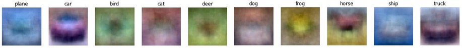
There are two complementary ways to understand what the weight vector \(\mathbf{w}\) actually learns. The first is template matching (from CS231n, Stanford).
Think of \(\mathbf{w}\) as a learned prototype or template for the positive class. The raw score is simply an inner product:
A large positive \(s\) means \(\mathbf{x}\) is highly aligned with the template \(\mathbf{w}\) — the input looks like the learned prototype. A large negative \(s\) means \(\mathbf{x}\) is anti-aligned — it looks like the opposite class. This is conceptually similar to nearest-neighbor classification, but instead of comparing against every training example we compare against a single learned prototype per class.
4. Interpreting the Linear Classifier: Geometric View
The second interpretation is geometric. The score \(s = \mathbf{w}^\top \mathbf{x} + b\) is a linear function over feature space, and its geometry directly reveals what the classifier is doing.
- The set of all points where \(s = 0\) is the decision boundary — a hyperplane (a line in 2D).
- The weight vector \(\mathbf{w}\) is perpendicular to this hyperplane and points toward the positive class. Moving along \(\mathbf{w}\) increases the score; moving against it decreases it.
- The bias \(b\) shifts the hyperplane away from the origin. Without it, every decision boundary is forced through the origin — a severe restriction that prevents the model from fitting data that is not origin-centered.
5. The Sigmoid Function
Rather than a hard threshold, we often want a smooth probability estimate. The sigmoid function maps any real number to \((0,1)\):
Key properties:
- \(\sigma(0) = 0.5\) — at the decision boundary, the model is 50/50.
- \(\sigma(s) \to 1\) as \(s \to +\infty\) — large positive scores → confident class 1.
- \(\sigma(s) \to 0\) as \(s \to -\infty\) — large negative scores → confident class 0.
- \(\sigma'(s) = \sigma(s)(1-\sigma(s))\) — a handy identity for backprop.
Figure: The sigmoid function \(\sigma(s) = 1/(1+e^{-s})\). The gold dot marks \(\sigma(0) = 0.5\).
We define the predicted probability as \(\hat{p} = \sigma(\mathbf{w}^\top \mathbf{x} + b)\).
6. From Binary to Multi-Class: The Softmax Function
The sigmoid function works perfectly for binary classification (two classes). When there are \(K > 2\) classes, we need to produce \(K\) probabilities — one per class — that are all positive and sum to 1. The softmax function does exactly this.
Given a vector of \(K\) raw scores \(\mathbf{s} = [s_1, s_2, \ldots, s_K]^\top\), softmax returns a probability vector:
Key properties:
- \(P_k > 0\) for all \(k\) — exponential is always positive.
- \(\sum_{k=1}^{K} P_k = 1\) — the outputs form a valid probability distribution.
- The class with the largest score receives the highest probability.
- Adding a constant to all scores leaves the probabilities unchanged (only differences matter).
In the multi-class linear classifier, a separate weight vector is learned for each class. These are stacked into a weight matrix \(\mathbf{W} \in \mathbb{R}^{K \times d}\):
For a batch of \(N\) examples packed into a matrix \(\mathbf{X} \in \mathbb{R}^{d \times N}\), the entire forward pass is:
Z = Z - max(Z, [], 1); before exp(Z).
7. Loss Functions
A loss function \(L(\hat{y}, y)\) quantifies how wrong the model's prediction is. We want to minimize the average loss over all training examples.
7a. Mean Squared Error (MSE) — for regression
MSE is the natural loss for regression. It penalizes large errors quadratically. However, for classification it has poor gradient behavior — the loss can saturate when the sigmoid output is near 0 or 1.
7b. Binary Cross-Entropy — for binary classification
Cross-entropy has two key advantages over MSE for classification:
- Probabilistic interpretation: it is the negative log-likelihood under a Bernoulli model.
- Better gradients: when the model is confidently wrong, cross-entropy provides a large gradient signal to correct it quickly.
| \(i\) | Object | \(y_i\) (true label) | \(\hat{p}_i\) (predicted prob. of satellite) | Loss term |
|---|---|---|---|---|
| 1 | Satellite | 1 | 0.90 | \(-\log(0.90) \approx 0.105\) ✓ low |
| 2 | Debris | 0 | 0.15 | \(-\log(1-0.15) \approx 0.163\) ✓ low |
| 3 | Satellite | 1 | 0.08 | \(-\log(0.08) \approx 2.526\) ✗ high |
\(L_\text{BCE} = \tfrac{1}{3}(0.105 + 0.163 + 2.526) \approx 0.931\)
Notice: when \(y_i = 1\), only the \(\log(\hat{p}_i)\) term matters (the \((1-y_i)\) factor zeros out the other term). When \(y_i = 0\), only the \(\log(1-\hat{p}_i)\) term matters. Object 3 — a satellite the model nearly called debris — dominates the loss and will receive the largest gradient correction.
7c. Multi-class Cross-Entropy — for softmax classifiers
When there are \(K\) classes, the binary cross-entropy generalizes naturally. The true label for each example is represented as a one-hot vector \(\mathbf{y} \in \{0,1\}^K\) with a 1 in the position of the correct class and 0s elsewhere. The multi-class cross-entropy loss is:
Because \(y_{kn}\) is one-hot, only one term in the inner sum is nonzero for each example — the term corresponding to the true class. So the loss simplifies to:
i.e., the average negative log-probability assigned to the correct class. When \(K = 2\) and the labels are one-hot \([y, 1-y]^\top\), this reduces exactly to the binary cross-entropy in section 7b.
8. The Big Picture: Logistic & Softmax Regression
The components covered in this lesson combine into two closely related models:
| Binary (2 classes) | Multi-class (\(K\) classes) | |
|---|---|---|
| Scores | \(s = \mathbf{w}^\top\mathbf{x} + b\) | \(\mathbf{s} = \mathbf{W}\mathbf{x} + \mathbf{b}\) |
| Activation | Sigmoid \(\sigma(s)\) | Softmax \(P_k = e^{s_k}/\sum e^{s_j}\) |
| Loss | Binary cross-entropy | Multi-class cross-entropy |
| Name | Logistic regression | Softmax regression |
In both cases we find \(\boldsymbol{\theta}\) that minimizes \(L\). This requires a numerical optimization method — that is the subject of Lesson 35.
Recommended Video
Two recommended videos — StatQuest for a step-by-step derivation of logistic regression and cross-entropy, and CS231n Lecture 2 for the broader linear classification framework covered in this lesson:
MATLAB Tips & Tricks
Building a One-Hot Label Matrix
Many classifiers require labels as a one-hot matrix \(\mathbf{Y}\) rather than a vector of integers. If ID is an \(N \times 1\) vector of class labels (integers 1–K), you need a \(K \times N\) matrix where column \(n\) has a 1 in row ID(n) and zeros everywhere else.
Two common approaches in MATLAB:
Option 1 — Using ind2vec (requires Neural Network Toolbox)
% ID is N×1, e.g. [1; 3; 2; 4; 1]
% ind2vec expects a row vector, so transpose first
Y_oh = full(ind2vec(ID'));   % K × N one-hot matrix
% full() converts the sparse output to a regular dense matrix
Option 2 — Manual construction (no toolbox required)
K = 4;   % number of classes
N = length(ID);
Y_oh = zeros(K, N);
for n = 1:N
    Y_oh(ID(n), n) = 1;
end
Option 3 — Using logical indexing with eye (compact, no toolbox)
% eye(K) is the K×K identity matrix — each column is already one-hot.
% Indexing its columns by ID selects the right one-hot vector for each object.
K = 4;
Y_oh = eye(K)(:, ID); % K × N one-hot matrixY_oh should sum to 1, and the row index of the 1 in column n should equal ID(n). A quick check: all(sum(Y_oh,1) == 1) should return true, and [~, rows] = max(Y_oh) should reproduce ID'.
Summary
| Concept | Formula / Key Idea |
|---|---|
| Linear score | \(s = \mathbf{w}^\top \mathbf{x} + b\) |
| Decision boundary | Hyperplane \(\mathbf{w}^\top \mathbf{x} + b = 0\) |
| Sigmoid | \(\sigma(s) = 1/(1+e^{-s})\), maps \(\mathbb{R} \to (0,1)\) — binary |
| Softmax | \(P_k = e^{s_k}/\sum_j e^{s_j}\), maps \(\mathbb{R}^K \to \Delta^{K-1}\) — multi-class |
| MSE loss | \(\frac{1}{N}\sum(\hat{y}-y)^2\) — for regression |
| Binary cross-entropy | \(-\frac{1}{N}\sum[y\log\hat{p} + (1-y)\log(1-\hat{p})]\) |
| Multi-class cross-entropy | \(-\frac{1}{N}\sum_n\sum_k y_{kn}\log P_{kn}\) |
| Logistic regression | Linear score + sigmoid + binary CE (2 classes) |
| Softmax regression | Linear scores + softmax + multi-class CE (\(K\) classes) |
References
- Goodfellow, I., Bengio, Y., & Courville, A. (2016). Deep Learning, Ch. 6. MIT Press.
- Karpathy, A., Johnson, J., & Li, F.-F. (2017). CS231n: Convolutional Neural Networks for Visual Recognition — Lecture 2 notes: Linear Classification. Stanford University. cs231n.github.io/linear-classify
- StatQuest. (2019). Logistic Regression [Video series]. YouTube.
- Bishop, C. M. (2006). Pattern Recognition and Machine Learning, Ch. 4. Springer.
- Ng, A. (2012). Machine Learning (Coursera lecture notes). Stanford University.