Lesson 30 — Gradient-Based Optimization

Learning Objectives

Explain why GSS cannot be generalized to multidimensional functions.
Define the gradient as a vector of partial derivatives and interpret its magnitude and direction.
Compute gradients analytically and evaluate them at specific points.
Implement the gradient descent (GD) update rule and explain the role of step size \(\gamma\).
Describe the steepest descent (SD) algorithm and how it selects the optimal \(\gamma\) at each step.
Apply a convergence criterion based on the L2 norm of successive iterates.
Implement GD as a MATLAB UDF that accepts a function handle and gradient handle.

Notation used in this lesson

\(f(x)\)Scalar function to minimize (\(x\) is a vector)

\(\nabla f(x)\)Gradient vector of \(f\) at \(x\)

\(x^k\)Current estimate of the minimum at iteration \(k\)

\(\gamma\)Step size (scalar; fixed in GD, optimized in SD)

\(\gamma^k\)Optimal step size at iteration \(k\) (SD only)

\(\epsilon\)Convergence threshold

\(\|\cdot\|_2\)Euclidean (L2) norm: \(\|v\|_2 = \sqrt{v^T v}\)

\(\partial f / \partial x_i\)Partial derivative with respect to \(x_i\)

🌐 Why We Need a New Approach

Golden Section Search is robust and efficient for one-dimensional functions, but it cannot be extended to higher dimensions. There is no multidimensional analogue of "the interval containing the minimum shrinks from both ends." A 2D function has infinitely many directions to explore, and bracketing along all of them simultaneously is impractical.

Many important physics and engineering problems involve minimizing functions of many variables — the energy of a molecular configuration (\(3N\) coordinates), the parameters of a fitted model, or the weights of a neural network. We need an approach that scales.

Key insight: The gradient \(\nabla f(x)\) points in the direction of steepest increase. Moving in the opposite direction — against the gradient — moves downhill toward the minimum. This is the foundation of all gradient-based optimization.

∇ Gradient Review

Definition

The gradient is the multivariable generalization of the derivative. For a scalar function \(f(x)\) of an \(n\)-dimensional vector \(x = [x_1, x_2, \ldots, x_n]^T\), the gradient is the column vector of partial derivatives:

\nabla f(x) = \begin{bmatrix} \dfrac{\partial f}{\partial x_1} \\[8pt] \dfrac{\partial f}{\partial x_2} \\ \vdots \\ \dfrac{\partial f}{\partial x_n} \end{bmatrix}

The gradient is itself a function of position \(x\). It has both a magnitude (how steep the function is at that point) and a direction (pointing toward the greatest rate of increase). At a minimum, the gradient is zero: \(\nabla f(x^*) = 0\).

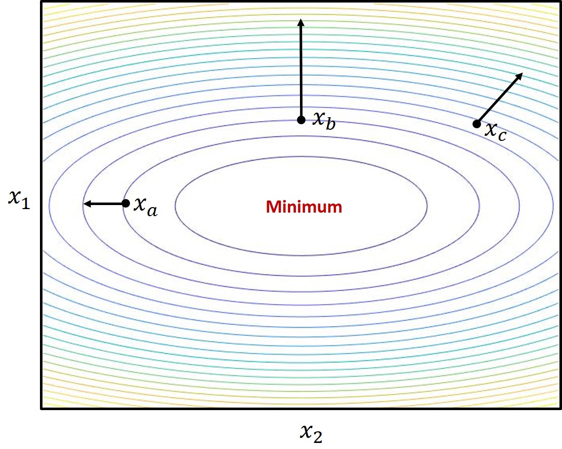
Example: \(f(x) = 4x_1^2 + x_2^2\)

This 2D quadratic has a minimum at the origin. Its gradient is:

\nabla f(x) = \begin{bmatrix} 8x_1 \\ 2x_2 \end{bmatrix}

Evaluating at three points:

Point \(x\)	Gradient \(\nabla f(x)\)	Interpretation
\([0,\ -1]^T\)	\([0,\ -2]^T\)	Pointing straight down — move up to reach minimum
\([-1,\ 0]^T\)	\([-8,\ 0]^T\)	Pointing left — move right
\([-1,\ 1]^T\)	\([-8,\ 2]^T\)	Pointing left and up — move right and down

Contour plot intuition: On a contour plot, the gradient is always perpendicular to the contour lines and points toward higher contour values. Moving against the gradient — inward toward the center — moves toward lower values and the minimum.

Contour plot showing gradient vectors at three points perpendicular to contour lines — **Figure 1.** Contour plot of a 2D function. At three sample points \(x_a\), \(x_b\), and \(x_c\), the gradient \(\nabla f\) is drawn as an arrow. In every case the arrow is *perpendicular to the local contour line* and points toward higher function values (away from the minimum). Gradient descent moves each iterate in the *opposite* direction — along \(-\nabla f\) — to descend toward the minimum.

📐 Gradient Descent (GD)

Update rule

The gradient descent algorithm starts at an initial point \(x^0\) and repeatedly moves in the direction opposite the gradient:

x^{k+1} = x^k - \gamma\, \nabla f(x^k)

where \(k\) is the iteration number and \(\gamma > 0\) is the step size (also called the learning rate). Because \(x\) and \(\nabla f\) are both vectors, this is a vector subtraction: each component of \(x\) is updated by a step proportional to the corresponding partial derivative.

The challenge of choosing \(\gamma\)

The step size \(\gamma\) is fixed for all iterations in basic GD and must be chosen carefully:

\(\gamma\) too small: The algorithm makes tiny steps and converges very slowly — or may never reach the minimum within a practical number of iterations.
\(\gamma\) too large: Each step overshoots the minimum. The algorithm bounces back and forth across the minimum and may diverge entirely.
\(\gamma\) just right: The algorithm converges steadily to the minimum.

There is no universal rule for choosing \(\gamma\). It depends on the curvature of \(f\). In practice, \(\gamma\) is treated as a hyperparameter: try a few values, monitor convergence, and adjust. Despite this challenge, GD is widely used — including in almost every neural network training algorithm.

🎯 Steepest Descent (SD)

Optimal step size per iteration

Steepest descent uses the same update rule as GD, but instead of a fixed \(\gamma\), it finds the optimal step size at each iteration. The optimal \(\gamma^k\) is the one that produces the maximum decrease in \(f\) along the current gradient direction:

\gamma^k = \underset{\gamma}{\operatorname{argmin}} \left\{ f\!\left( x^k - \gamma\, \nabla f(x^k) \right) \right\}

Note that \(f\bigl(x^k - \gamma\,\nabla f(x^k)\bigr)\) is a scalar function of the scalar variable \(\gamma\) only — \(x^k\) is the known current position, not a variable. This is a 1D optimization problem, which can be solved with GSS from Lesson 29.

Why this is better in principle: Each SD step is guaranteed to make the largest possible decrease for the given gradient direction. No tuning of \(\gamma\) is required.

Why GD is often used instead: Solving a 1D optimization (GSS) at every iteration adds significant computational overhead. For large-scale problems (e.g., neural networks with millions of parameters), this cost dominates the total runtime. Fixed-\(\gamma\) GD, despite requiring careful tuning, is usually faster in practice.

🔁 Convergence and Stopping Criteria

Why convergence is not guaranteed

Gradient-based algorithms follow the local downhill path, regardless of whether it leads to the global minimum. Starting from a different \(x^0\) may lead to a different local minimum. For non-convex functions, the initial point matters.

As the algorithm approaches a minimum, \(\nabla f(x^k) \to 0\), so the update steps \(x^{k+1} - x^k = -\gamma\nabla f(x^k)\) also shrink toward zero. The algorithm slows down near the minimum — this is expected and not a sign of failure.

Stopping condition

A practical stopping rule is to halt when the change in position between consecutive iterates falls below a threshold \(\epsilon\):

\| x^k - x^{k-1} \|_2 \leq \epsilon

where the L2 (Euclidean) norm of a vector \(v\) is

\| v \|_2 = \sqrt{v^T v} = \sqrt{\sum_i v_i^2}.

Alternative stopping rules include checking the magnitude of the gradient (\(\|\nabla f\|_2 \leq \epsilon\)) or the change in function value (\(|f^k - f^{k-1}| \leq \epsilon\)). All three are reasonable; in MATLAB, norm(x_new - x_old) computes the L2 norm directly.

▶ Recommended Video

Dr. Trefor Bazett derives gradient descent directly from the directional derivative and multivariable calculus — framed as a general minimization method for high-dimensional functions, with no machine learning context.

▶

Intro to Gradient Descent || Optimizing High-Dimensional Equations

Dr. Trefor Bazett — YouTube

💻 Numerical Walkthrough — MATLAB

The script below manually steps through 5 iterations of gradient descent on \(f(x_1,x_2) = 4x_1^2 + x_2^2\) starting from \(x^0 = [1.5,\,1.5]^T\) with \(\gamma = 0.10\). Each step is written out explicitly so you can see exactly what the algorithm does. The true minimum is at \(x^* = [0,\,0]^T\).

%% Lesson 30 — GD: Hard-Coded 5-Step Walkthrough
% f(x1,x2) = 4*x1^2 + x2^2,   minimum at x* = [0; 0]
% grad f  =  [8*x1; 2*x2]
% Start: x0 = [1.5; 1.5],   gamma = 0.10

f      = @(x) 4*x(1)^2 + x(2)^2;
grad_f = @(x) [8*x(1); 2*x(2)];
gamma  = 0.10;

%% ── Step 0: evaluate gradient at x0, take one step ───────────────────────
x0 = [1.5; 1.5];
g0 = grad_f(x0);          % g0 = [12.0000;  3.0000]
x1 = x0 - gamma*g0;       % x1 = [ 0.3000;  1.2000]
fprintf('x0=[%7.4f, %7.4f]   f=%7.4f   |g|=%7.4f\n', x0(1),x0(2),f(x0),norm(g0))

%% ── Step 1 ────────────────────────────────────────────────────────────────
g1 = grad_f(x1);          % g1 = [ 2.4000;  2.4000]
x2 = x1 - gamma*g1;       % x2 = [ 0.0600;  0.9600]
fprintf('x1=[%7.4f, %7.4f]   f=%7.4f   |g|=%7.4f\n', x1(1),x1(2),f(x1),norm(g1))

%% ── Step 2 ────────────────────────────────────────────────────────────────
g2 = grad_f(x2);          % g2 = [ 0.4800;  1.9200]
x3 = x2 - gamma*g2;       % x3 = [ 0.0120;  0.7680]
fprintf('x2=[%7.4f, %7.4f]   f=%7.4f   |g|=%7.4f\n', x2(1),x2(2),f(x2),norm(g2))

%% ── Step 3 ────────────────────────────────────────────────────────────────
g3 = grad_f(x3);          % g3 = [ 0.0960;  1.5360]
x4 = x3 - gamma*g3;       % x4 = [ 0.0024;  0.6144]
fprintf('x3=[%7.4f, %7.4f]   f=%7.4f   |g|=%7.4f\n', x3(1),x3(2),f(x3),norm(g3))

%% ── Step 4 ────────────────────────────────────────────────────────────────
g4 = grad_f(x4);          % g4 = [ 0.0192;  1.2288]
x5 = x4 - gamma*g4;       % x5 = [0.00048; 0.49152]
fprintf('x4=[%7.4f, %7.4f]   f=%7.4f   |g|=%7.4f\n', x4(1),x4(2),f(x4),norm(g4))
fprintf('\nAfter 5 steps: x5=[%.5f; %.5f]   f=%.4f\n', x5(1),x5(2),f(x5))
fprintf('True x* = [0; 0],  f(x*) = 0\n')

%% ── Plots ─────────────────────────────────────────────────────────────────
pts   = [x0, x1, x2, x3, x4, x5];   % 2x6 matrix of all iterates
grads = [g0, g1, g2, g3, g4];        % 2x5 matrix of gradients at x0..x4

figure('Position', [100 100 1100 440])

%% Panel 1: contour + GD path + gradient arrows
subplot(1,2,1)
[X1,X2] = meshgrid(linspace(-0.3,1.8,200), linspace(-0.2,1.7,200));
F = 4*X1.^2 + X2.^2;
contourf(X1,X2,F,14,'LineColor','none');   hold on
contour(X1,X2,F,14,'k','LineWidth',0.4)
colorbar

% White connecting path (no legend entry)
plot(pts(1,:), pts(2,:), 'w-', 'LineWidth', 1.5, 'HandleVisibility','off')

% Color palette — one color per iterate x0..x5
clr = [0.55 0.55 0.55;   % gray   x0
       0.00 0.45 0.74;   % blue   x1
       0.85 0.33 0.10;   % orange x2
       0.47 0.67 0.19;   % green  x3
       0.49 0.18 0.56;   % purple x4
       0.64 0.08 0.18];  % red    x5

% Plot each iterate
for k = 1:6
    plot(pts(1,k), pts(2,k), 'o', 'MarkerSize', 9, ...
         'Color', clr(k,:), 'MarkerFaceColor', clr(k,:), ...
         'DisplayName', sprintf('$x_%d$', k-1))
end

% Gradient arrows — normalized to fixed visual length (direction only)
alen = 0.18;
for k = 1:5
    ghat = grads(:,k) / norm(grads(:,k));
    quiver(pts(1,k), pts(2,k), alen*ghat(1), alen*ghat(2), 0, ...
           'Color', clr(k,:), 'LineWidth', 1.8, 'MaxHeadSize', 0.6, ...
           'HandleVisibility','off')
end

% Dummy quiver for legend
hq = quiver(NaN, NaN, NaN, NaN, 'k-', 'LineWidth', 1.5);
hq.DisplayName = '$\nabla f$ (unit dir.)';

% True minimum
plot(0, 0, 'kp', 'MarkerSize', 14, 'MarkerFaceColor', 'k', 'DisplayName', '$x^*$')

xlabel('$x_1$', 'Interpreter', 'latex');   ylabel('$x_2$', 'Interpreter', 'latex')
title('GD path: $f = 4x_1^2 + x_2^2$,  $\gamma = 0.10$', 'Interpreter', 'latex')
legend('Location', 'southeast', 'Interpreter', 'latex');   grid on

%% Panel 2: f(x^k) vs. iteration (semilog)
subplot(1,2,2)
fvals = [f(x0), f(x1), f(x2), f(x3), f(x4), f(x5)];
semilogy(0:5, fvals, 'ko-', 'LineWidth', 1.8, 'MarkerFaceColor','k')
xlabel('Iteration');   ylabel('$f(x^k)$', 'Interpreter', 'latex')
title('$f(x^k)$ vs. iteration', 'Interpreter', 'latex')
grid on

sgtitle('GD Walkthrough: $f = 4x_1^2 + x_2^2$,  $\gamma=0.10$,  $x_0=[1.5;\,1.5]$', 'Interpreter', 'latex')

What to notice: The \(x_1\) component converges in roughly 2 steps (decay factor \(1-\gamma\cdot8=0.2\) per step) while \(x_2\) decays slowly (factor \(1-\gamma\cdot2=0.8\)). This ill-conditioning — different curvatures in different directions — is what causes the elongated, funnel-shaped path. The gradient arrows are normalized to unit length to show direction; the actual gradient magnitude shrinks with each step.

HW 30 asks you to write a general-purpose GD UDF that accepts function and gradient handles, and apply it to a different 2D function with its minimum away from the origin.

📝 Summary

Concept	Key Idea
Gradient \(\nabla f\)	Vector of partial derivatives; points toward steepest increase; zero at a minimum.
Gradient Descent	\(x^{k+1} = x^k - \gamma\nabla f(x^k)\); fixed step size \(\gamma\) for all iterations.
Step size \(\gamma\)	Too small → slow; too large → diverges. Must be tuned per problem.
Steepest Descent	Same update rule, but \(\gamma^k\) is optimized at each step via 1D GSS.
SD trade-off	Guaranteed maximum decrease per step, but 1D optimization at each iteration is expensive.
Stopping criterion	\(\\|x^k - x^{k-1}\\|_2 \leq \epsilon\); stop when steps become negligible.
Local vs. global	Both GD and SD converge to a local minimum; starting point matters for non-convex \(f\).

📋 HW 30 — Gradient Descent UDF

📚 References

Pellizzari, C.A. Physics 356 — Supplement on Gradient-Based Optimization, USAFA, 2021.
Bouman, C.A. Foundations of Computational Imaging, SIAM, 2022.
Chong, E.K.P. and Zak, S.H. An Introduction to Optimization, 4th Ed., John Wiley & Sons, 2013, pp. 123–124.
Wikipedia contributors. "Gradient." Wikipedia, The Free Encyclopedia, 2019.

← Previous
L29: Bracketing & GSS

Next Lesson
L31: Maximum Likelihood Estimation

→

Gradient-Based Optimization: Gradient Descent & Steepest Descent

Learning Objectives

Notation used in this lesson

🌐 Why We Need a New Approach

∇ Gradient Review

Definition

Example: \(f(x) = 4x_1^2 + x_2^2\)

📐 Gradient Descent (GD)

Update rule

The challenge of choosing \(\gamma\)

🎯 Steepest Descent (SD)

Optimal step size per iteration

🔁 Convergence and Stopping Criteria

Why convergence is not guaranteed

Stopping condition

▶ Recommended Video

💻 Numerical Walkthrough — MATLAB

📝 Summary

📚 References